2 Data

2.1 Description

The data source for this project is the “NYPD Arrest Data (Year to Date)” dataset, available through NYC OpenData. This data is collected by the New York Police Department (NYPD) and is reviewed by the Office of Management Analysis and Planning. Each record represents an arrest made in NYC by the NYPD, including details such as the type of crime, location, time of enforcement, and perpetrator’s demographics.

The data is in tabular format, consisting of 19 columns and approximately 195,000 rows, and is manually updated every quarter, with the data format including both numerical and text categorical fields. The available attachment, “NYPD_Arrest_YTD_DataDictionary.xlsx,” contains a detailed description of each variable.

However, the dataset has several potential issues, including inconsistencies or delays due to manual updates, and outdated entries because of the quarterly update frequency. Null values are frequently present in certain fields, as some specific data were not collected or were unknown at the time of the report. Additionally, geo-location inaccuracies may affect spatial analysis since some arrests are represented by approximate coordinates.

The dataset is available in CSV format on the NYC OpenData portal, which can be directly exported, downloaded locally, and imported into RStudio using the read.csv() function.

2.2 Missing value analysis

Code

library(ggplot2)
library(dplyr)
library(tidyr)
library(naniar)

Code

data <- read.csv("NYPD_Arrest_Data.csv", na.strings = c("(null)", "N/A"))
missing_summary <- data |>
  summarise(across(everything(), ~ sum(is.na(.)))) |>
  pivot_longer(cols = everything(), names_to = "Column", values_to = "Missing_Values") |>
  arrange(desc(Missing_Values)) |>
  mutate(Column = factor(Column, levels = Column)) |>
  mutate(Proportion = Missing_Values / nrow(data)) 

ggplot(missing_summary, aes(x = Column, y = Missing_Values)) +
  geom_bar(stat = "identity", fill = "blue") +
  labs(title = "Number and Proportion of Missing Values by Column", x = "Columns", y = "Number of missing values") +
  theme(axis.text.x = element_text(angle = 45, hjust = 1)) +
  scale_y_continuous(
    name = "Number of missing values",
    sec.axis = sec_axis(~ . / nrow(data) * 100, name = "Proportion of missing values (%)")
  )

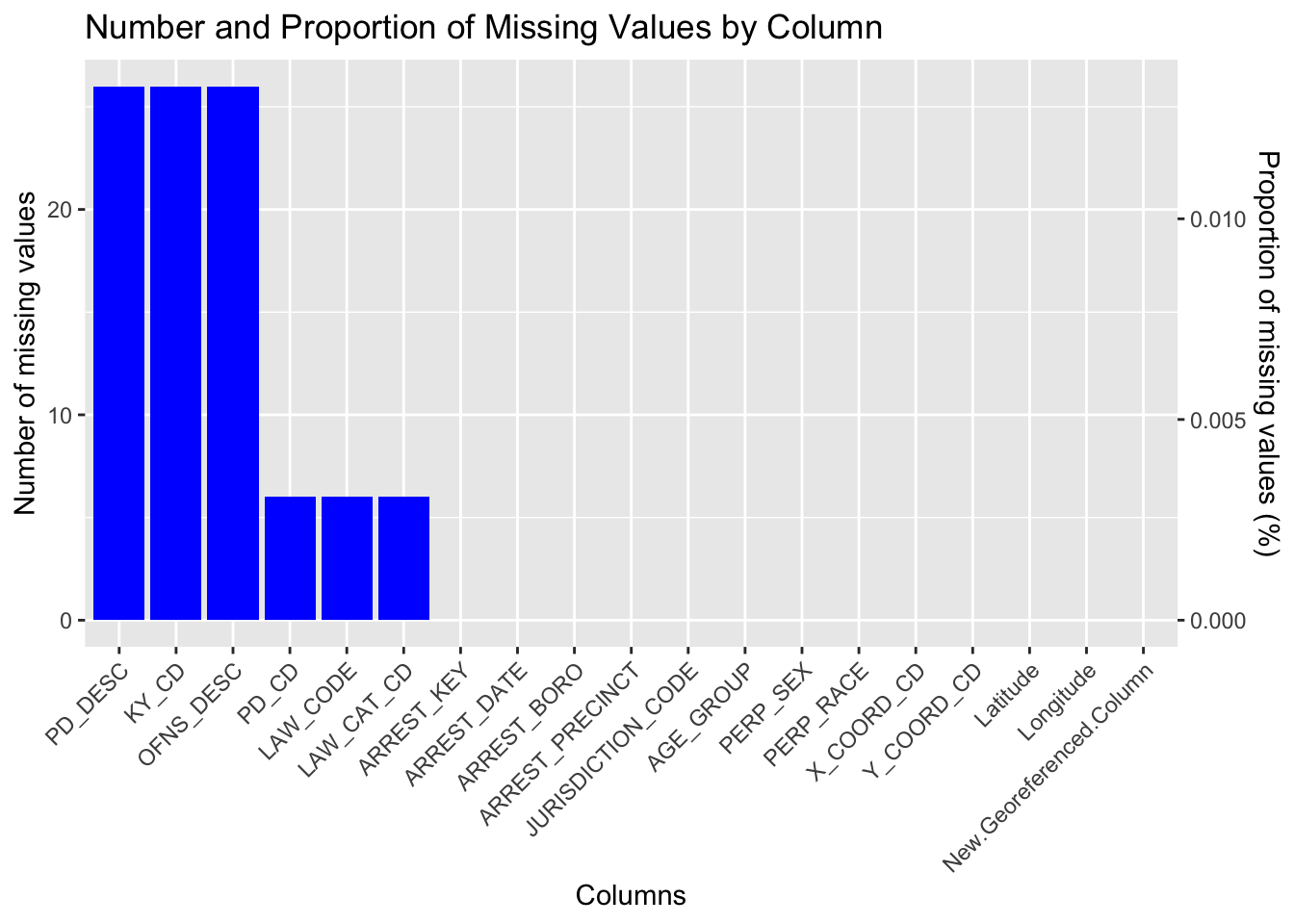
The columns PD_DESC, KY_CD, and OFNS_DESC have the highest number of missing values (26 rows each) and the columns PD_CD, LAW_CODE, and LAW_CAT_CD have fewer missing values (6 rows each). All other columns have no missing values. This discrepancy arises because certain data, like the arrest date, borough of arrest and perpetrator’s demographic information, are straightforward to record during the initial recording process. In contrast, classifying the level of offense and providing the description of internal classification often require more investigation or process.

The missing data in the dataset is negligible in the context of the overall dataset size, constituting less than 0.01%, indicating that the impact of missing data on analyses is minimal.

Code

data_with_na <- data |>
  filter(if_any(everything(), is.na))
vis_miss(data_with_na) +
  labs(title = "Heatmap of missing values across rows and columns", x = "Columns", y = "Rows")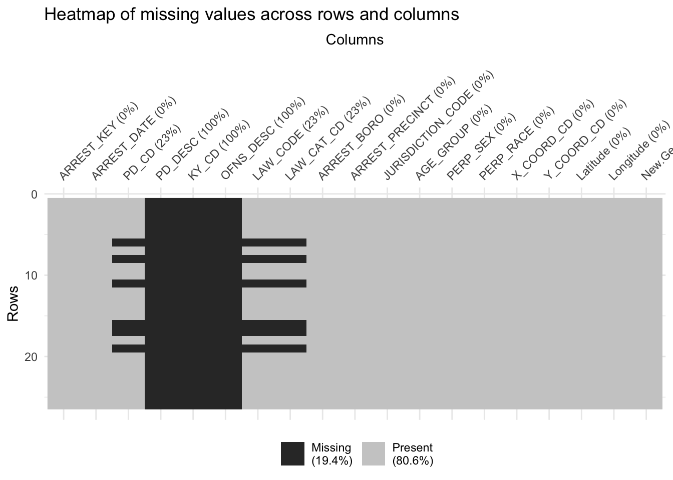

The heatmap reveals that missing values are concentrated in a few rows and specific columns, with no widespread gaps. This suggests missing data is likely due to specific incidents or cases rather than systemic issues. In particular, it might be the instances where information was not available or unknown at the time of the report.

Code

boro_na_summary <- data_with_na |>
  group_by(ARREST_BORO) |>
  summarise(Missing_Count = n()) |>
  arrange(desc(Missing_Count)) |>
    mutate(ARREST_BORO = case_when(
      ARREST_BORO == "B" ~ "Bronx",
      ARREST_BORO == "S" ~ "Staten Island",
      ARREST_BORO == "K" ~ "Brooklyn",
      ARREST_BORO == "M" ~ "Manhattan",
      ARREST_BORO == "Q" ~ "Queens"
    )) |>
  mutate(ARREST_BORO = factor(ARREST_BORO, levels = ARREST_BORO))
  
ggplot(boro_na_summary, aes(x = ARREST_BORO, y = Missing_Count)) +
  geom_bar(stat = "identity", fill = "lightblue") +
  scale_y_continuous(breaks = seq(0, 10, by = 2)) +
  labs(title = "Distribution of missing values by Arrest Borough", x = "Arrest Borough", y = "Count of Missing Rows")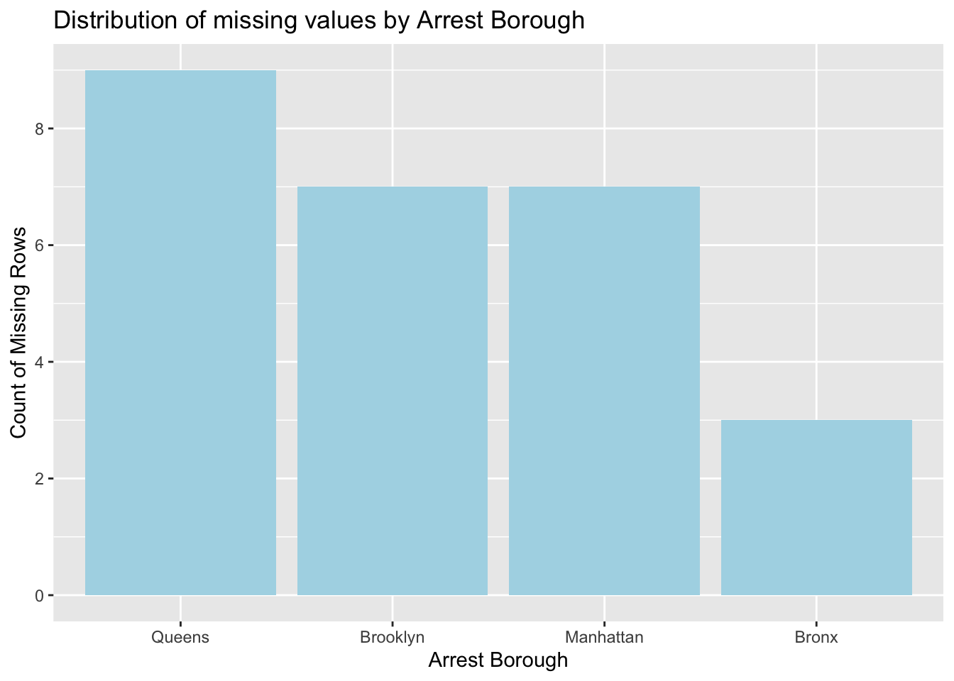

According to this bar plot, Queens has the highest number of missing values, followed by Brooklyn and Manhattan, while Bronx has the least. This distribution could reflect operational or reporting differences between boroughs.